Langevin Sampling for Diffusion Models

An overview of Langevin Sampling for Diffusion Models

Langevin Sampling for Diffusion Models

There are many resources on the internet that explain diffusion models as a noising and denoising process using a deep learning architecture. Although those are useful, most of them do not paint the whole picture. There’s another component that’s just as important as the deep learning part: the probabilistic framework that makes it all work .

Assigning Probability Values to Images

Imagine a black box called the image distribution. This box gives us samples from an underlying distribution — that is, images of all kinds.

These images have intrinsic likelihoods, similar to the rolling dice case. An image of a koala and an image of a tiger could have similar probabilities, while a noisy image would have much less likelihood:

\[p(\text{Koala}) \approx p(\text{Tiger}) > p(\text{Noise})\]

With this in mind, all we need to do is generate samples from this image distribution, right? But first, we need to understand how to generate samples from any distribution using a computer. Let’s start with a simpler case: how do we generate samples from a dice-rolling distribution?

Challenges in Sampling from Probability Distributions

Generating samples from a fair die is the simplest case. There are many libraries already implemented in Python that allow you to do this, such as random. But how would you implement it from first principles?

At first you might think that if we know the PMF of the probability distribution, then we’ll be able to generate samples from it. However, this is not exactly the case — we know how the PMF looks, but actually generating samples from it requires algorithms like the Mersenne Twister or Xorshift random number generators. This sounds kind of intimidating, so let’s look at an alternative approach.

Say we have a continuous uniform distribution and we can sample from it. Then:

1. Sample from the continuous uniform distribution:

\[x \sim \mathcal{U}(0, 1)\]

1. Threshold on multiples of $1/6$, which gives us the dice roll values:

\[\begin{align*} 0 < x < \frac{1}{6} &: \bullet \\ \frac{1}{6} < x < \frac{2}{6} &: \bullet\bullet \\ &\vdots \\ \frac{5}{6} < x < 1 &: \bullet\bullet\bullet\bullet\bullet\bullet \end{align*}\]

Interesting — although both of these are uniform distributions, so the trick feels a bit circular. However, there’s another distribution that, if we could sample from it, would allow us to sample from almost any other distribution.

The Probability Density Function with Two Peaks

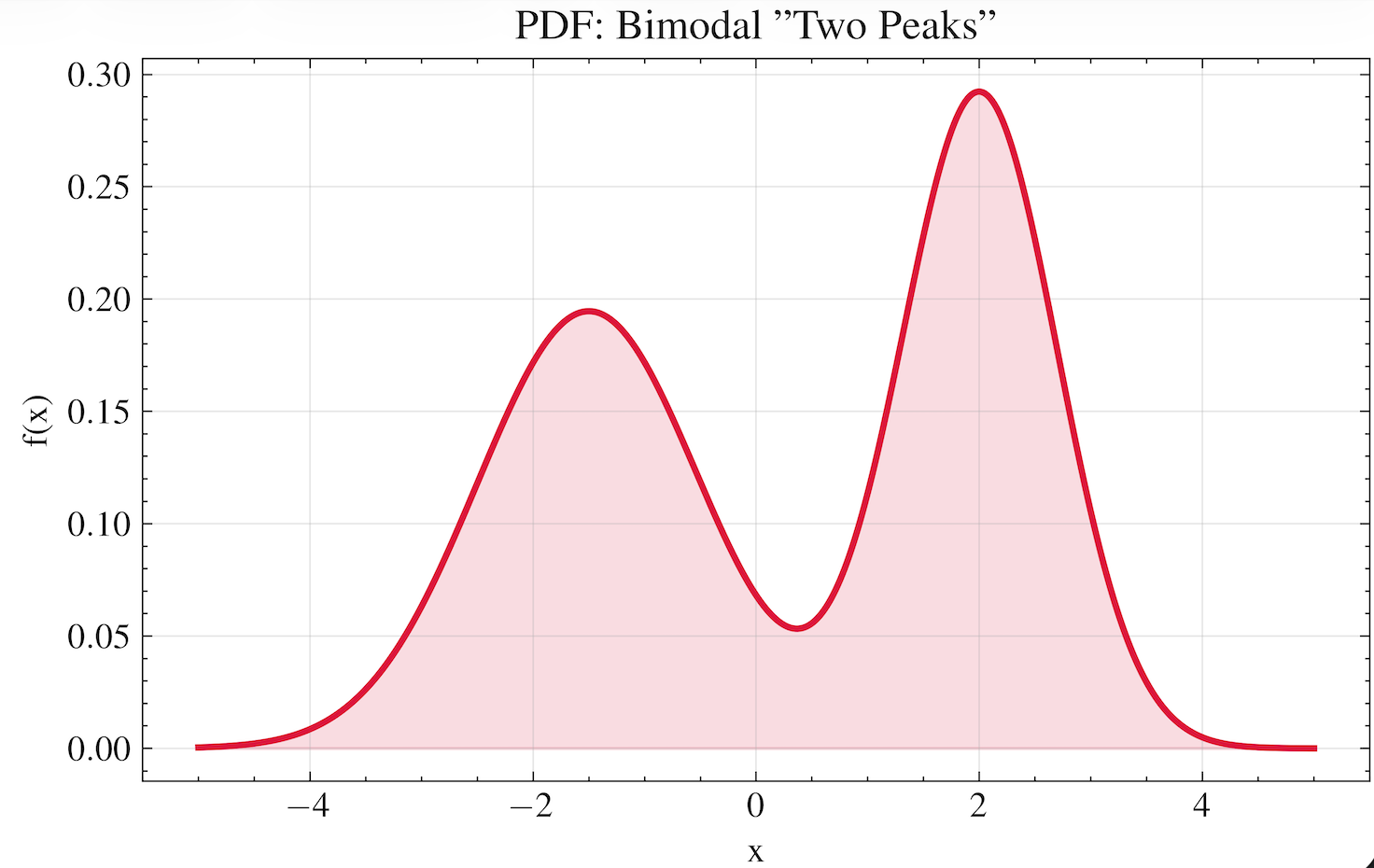
Let’s assume we have a PDF called $p_{\text{twopeaks}}(x)$ — a distribution with two distinct peaks.

The probability density function \( p_{\text{twopeaks}}(x) \) with two distinct peaks.

Also assume we have a function $F_{\text{twopeaks}}(x)$ which, given any input $x_i$, tells us whether we should move left or right to most quickly increase the value of $p_{\text{twopeaks}}(x)$.

Our third assumption is that we can generate samples from a normal distribution.

With all three assumptions in place, we can begin.

Langevin Sampling: An Algorithm That Generates Samples from Any Probability Distribution

Algorithm: Langevin sampling

\[\begin{array}{l} x_0 \sim \mathcal{N}(0, 1) \\ \textbf{for } t = 0 \text{ to } 1000: \\ \quad z_t \sim \mathcal{N}(0, 1) \\ \quad x_{t+1} = x_t + \epsilon F(x_t) + \sqrt{2\epsilon} z_t \\ \textbf{return } x_{1000} \end{array}\]

Langevin Sampling algorithm: iteratively applying gradient-based updates with Gaussian noise to generate samples from a target distribution.

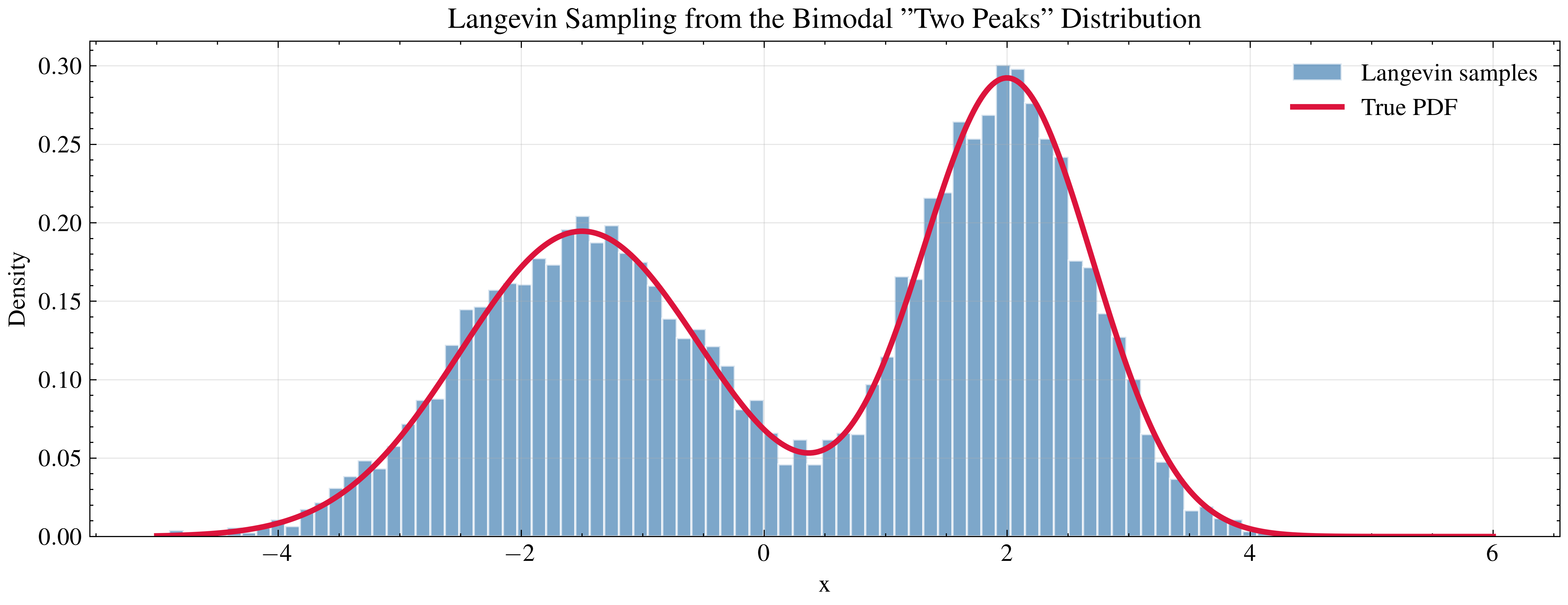
The Langevin Sampling algorithm is described in the image above. One iteration in the loop is called a Langevin Update. We iterate thousands of times (say 1,000) to generate a single sample. Then we repeat this entire process many times to build up a histogram that approximates the target distribution.

It’s important that we add Gaussian noise at each iteration to prevent the sample from collapsing onto the peak itself. The randomness is essential — it keeps the deterministic gradient ascent from getting stuck.

Intuition for the Score Function

Now, let’s look at the $F$ term — the score function. It’s defined as:

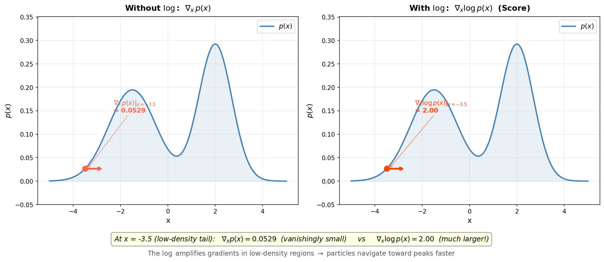
\[F(x_t) = \nabla_x \log p(x_t)\]

It’s intuitive that this gradient (derivative) gives us the direction of quickest increase. But why the $\log$?

The logarithm amplifies the magnitude of the gradient in low-density regions, allowing us to reach the most probable samples faster. Without it, the gradients in the tails of the distribution would be vanishingly small, making it hard to navigate toward the peaks.

Effect of the logarithm on the score function: amplifying gradients in low-density regions to improve navigation toward the peaks.

Now that we have that in place, let’s do an exercise: applying Langevin Sampling to generate samples from our dice-rolling setup. We’ll follow the strategy shown previously — first use Langevin Sampling to sample from a continuous uniform distribution (assuming we’re given a way to sample from a Gaussian distribution to perform the Langevin updates).

Exercise: A Dice Roll Sampler from Scratch Using Langevin Sampling

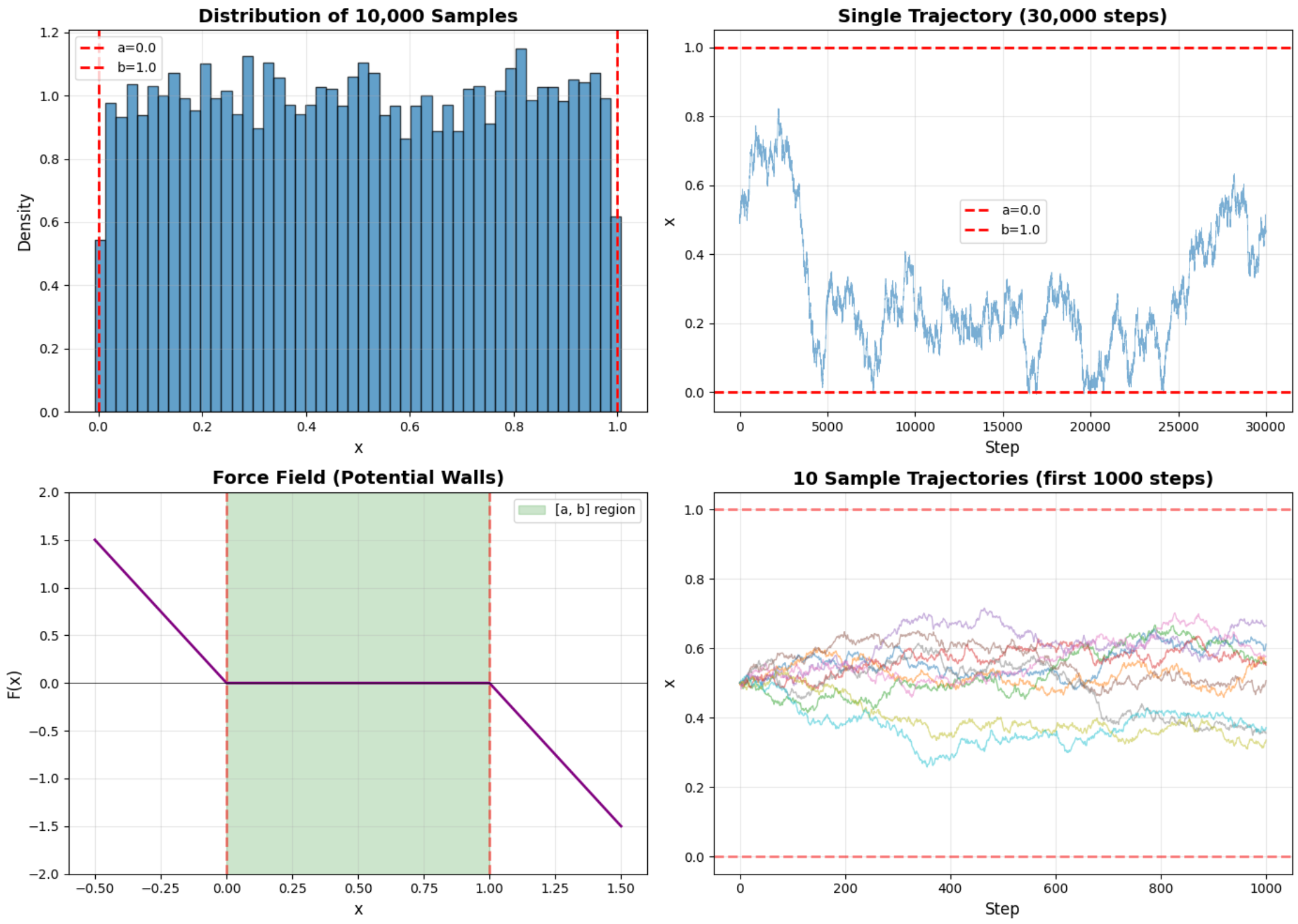
First, we need to obtain $F(x)$ for the uniform distribution in the correct sample space (from 0 to 1). If we take only the derivative, it would be zero everywhere inside the interval — not very helpful.

The derivative of the uniform distribution is zero everywhere inside the interval, requiring boundary "walls" to keep samples within the valid range.

However, this flat derivative could lead samples to drift outside the valid range, so we need to put “walls” that keep us inside the sample space we’re looking for. These walls act like a restoring force that pushes samples back when they wander outside $[0, 1]$.

Using this $F$ and the Gaussian distribution, we can generate samples from a uniform distribution. Then we apply the second step: threshold on multiples of $1/6$, and we have a generator of dice rolls built entirely from Langevin dynamics.

Generating samples from a uniform distribution using Langevin dynamics, then thresholding to produce dice rolls.

A Langevin Approach to Image Generation

If we were to sample from the PDF $p_{\text{image}}(\mathbf{x})$, where the sample space spans the dimension of all pixels in an image, it becomes much harder to visualize all possible combinations of those pixels. We need some way to obtain the score function of that PDF.

Visualizing score functions in higher dimensions

The score function can be visualized as a Vector Field that points in the direction of quickest increase of the PDF, with the length of each vector indicating the magnitude (the closer to the peak, the smaller the vector).

The major issue for our image PDF is that we don’t have an analytical expression for it:

\[\text{for } \mathbf{x} = \begin{bmatrix} x_1 \\ x_2 \\ \vdots \\ x_{1,000,000} \end{bmatrix}, \quad x_i \text{ is pixel } i \text{ of image } \mathbf{x}\] \[\begin{align*} p_{\text{images}}(\mathbf{x}) &= \text{ ?} \\ F_{\text{images}}(\mathbf{x}) &= \nabla_{\mathbf{x}} \log p_{\text{images}}(\mathbf{x}) = \text{ ?} \end{align*}\]

In the dice roll case, we did know the PDF of the uniform distribution, so we could compute $F$ by just reasoning about the sample space. But for images, the problem is much harder. However, there’s one advantage we do have: a collection of millions of images from the internet — which are samples from this very PDF.

Diffusion Models Estimate Unknown Score Functions from Existing Samples

A Diffusion Model learns the direction that points toward the closest cluster of good images (with a nuance I’ll address in the final section) — in other words, the score function we’ve been talking about.

This connects our Langevin Sampling approach with image generation. If we have the trained model providing the score function and this sampling technique, we can generate plausible images.

Why Add More Noise in the Denoising Process?

Similarly to the $p_{\text{twopeaks}}(x)$ example, if we don’t add noise during the iterative sampling, we get a blurry mess — which could be seen as the average of many images rather than a true sample from the distribution. The noise contributes to two things:

1. Diversity: it ensures the generated samples reflect the full probability distribution rather than collapsing to a single mode.
2. Exploration: it helps escape local optima, combating the short-sightedness of pure gradient ascent.

Noise as Part of a Team

The diffusion process and the noise can be seen as a two-person team: one logical, one creative. The work of both allows us to get realistic images. The purely logical component can’t generate a realistic image on its own — it needs randomness.

This is worth contrasting with Generative Adversarial Networks (GANs), which suffered from a problem known as mode collapse, where outputs became far less diverse than the true distribution.

Parallels with Stochastic Gradient Descent

Stochastic Gradient Descent does something remarkably similar. Instead of finding a peak (like Langevin Sampling), it finds a minimum — but the principle is the same. The “noise” in SGD isn’t added explicitly; it’s a natural consequence of using mini-batches of data, which makes the gradient inherently noisy. This method works incredibly well and is the foundation of deep learning during training. Langevin Sampling just extends this same idea of productive randomness to test time.

Final Nuances

There are a few important details I glossed over for the sake of clarity:

• Annealed Langevin Sampling: The model actually learns the score of the noised distribution at each noise level. Why? Because if we were to start from a noise sample and try to follow the score of the true (un-noised) distribution, it would be too sparse — you’d get lost. Instead, we add noise to give the score function meaningful signal, and then gradually reduce the noise level, annealing from high to low noise during sampling.

• Noise prediction ≈ Score estimation: During diffusion model training, the model learns to predict the added noise, and it’s not immediately obvious how this connects to the score function. Proving this equivalence is a topic for another post, but the short version is that predicting the noise is mathematically equivalent to estimating the score.

• Why does Langevin Sampling work at all? This question leans into statistical physics and stochastic calculus. The theoretical justification comes from the theory of Langevin dynamics and its connection to the Fokker-Planck equation. If you’re curious, that’s where to dig deeper.

Glossary

Probability Mass Function (PMF): For a discrete random variable $X$, the PMF $p_X(x)$ gives the probability that $X$ takes the value $x$:

\[p_X(x) = P(X = x)\]

where $\sum_{x \in \mathcal{X}} p_X(x) = 1$.

Probability Density Function (PDF): For a continuous random variable $X$, the PDF $f_X(x)$ describes the probability density at $x$. The probability that $X$ falls in an interval $[a, b]$ is:

\[P(a \leq X \leq b) = \int_a^b f_X(x) \, dx\]

where $\int_{-\infty}^{\infty} f_X(x) \, dx = 1$.

Score Function: The gradient of the log-probability density, $\nabla_x \log p(x)$. It points in the direction that most quickly increases the probability density.

Langevin Sampling: An iterative algorithm that generates samples from a target distribution using only the score function and Gaussian noise.

Mode Collapse: A failure mode in GANs where the generator produces only a small subset of the possible outputs, lacking diversity.